xray + dask: out-of-core, labeled arrays in Python

Xray provides labeled, multi-dimensional arrays. Dask provides a system for parallel computing. Together, they allow for easy analysis of scientific datasets that don’t fit into memory.

An introduction to xray

To make it easier to work with scientific data in Python, we researchers at The Climate Corporation wrote an open source library called xray. Xray provides data structures for multi-dimensional labeled arrays, building on NumPy and pandas. Our goal was to make it easier to work with labeled, gridded datasets from physical sensors and models. At Climate, we use it to analyze weather data and satellite images.

The key idea of xray is that it uses metadata in the form of labeled dimensions (e.g., “time”) and coordinate values (e.g., the date “2015-04-10”) to enable a suite of expressive, label based operations. Here’s a quick example of how we might manipulate a 3D array of temperature data with xray:

ds.sel(time='2014-12-11').max(['latitude', 'longitude'])

<xray.Dataset>
Dimensions:  (time: 4)
Coordinates:
  * time     (time) datetime64[ns] 2014-12-11 2014-12-11T06:00:00 ...
Data variables:
    t2m      (time) float64 311.4 316.2 312.0 309.6

For comparison, here’s the how we might write that using only NumPy:

# temperature contains 4x daily values for December 2014
# axis labels are (time, latitude, longitude)
ds.t2m.values[[40, 41, 42, 43]].max(axis=(1, 2));

Once we’ve done our computation, every xray dataset can be easily serialized to and from disk, using the portable and efficient netCDF file format (a dialect of HDF5):

ds.to_netcdf('my-dataset_.nc')
saved_ds = xray.open_dataset('my-dataset_.nc')
assert saved_ds.equals(ds)

Or you might pass your data off to pandas for further analysis in tabular form:

df = ds.to_dataframe()

Without a tool like xray, we would need to keep track of metadata manually in order to preserve it in operations and save it with our results when we’re done. This is burdensome, especially for exploratory analysis, so we often don’t bother. Even when metadata is present, without xray it’s often easier not to use the metadata directly in our code. Magic constants end up littering our scripts, like the numbers 1 and 2 in our NumPy example above. Implicit assumptions about our data are left in comments, or worse, are not even stated at all.

Xray provides short-term incentives for providing metadata, in the form of additional expressive power. But the real payoff is enhanced readability and reproducibility in the long term when you or a colleague come back to your code or data six months from now.

Loading medium-sized weather data with dask

Today I will talk about how we have extended xray to work with datasets that don’t fit into memory by integrating it with dask. Dask is a new Python library that extends NumPy to out-of-core datasets by blocking arrays into small chunks and executing on those chunks in parallel. It allows xray to easily process large data and also simultaneously make use of all of our CPU resources.

Weather data – especially models from numerical weather prediction – can be big. The world uses its biggest supercomputers to generate weather and climate forecasts that run on increasingly high resolution grids. Even for data analysis purposes, it’s easy to need to process 10s or 100s of GBs of data.

For this blog post, we’ll work with a directory of netCDF files downloaded from the European Centre for Medium-Range Weather Forecast’s ERA-Interim reanalysis with the new xray function to open a multi-file dataset, xray.open_mfdataset:

import numpy as np
import matplotlib.pyplot as plt
import xray

ds = xray.open_mfdataset('/Users/shoyer/data/era-interim/2t/*.nc', engine='scipy')
ds.attrs = {}  # for brevity, hide attributes

Previewing the dataset, we see that it consists of 35 years of 6-hourly surface temperature data at a spatial resolution of roughly 0.7 degrees:

ds

<xray.Dataset>
Dimensions:    (latitude: 256, longitude: 512, time: 52596)
Coordinates:
  * latitude   (latitude) &gt;f4 89.4628 88.767 88.067 87.3661 86.6648 ...
  * longitude  (longitude) &gt;f4 0.0 0.703125 1.40625 2.10938 2.8125 ...
  * time       (time) datetime64[ns] 1979-01-01 1979-01-01T06:00:00 ...
Data variables:
    t2m        (time, latitude, longitude) float64 240.6 240.6 240.6 ...

This is actually 51 GB of data once it’s uncompressed to 64-bit floats:

ds.nbytes * (2 ** -30)

51.363675981760025

Is this big data? No, not really; it fits on a single machine. But my laptop only has 16GB of memory, so I certainly could not analyze this dataset in memory.

The power of dask is that it enables analysis of “medium data” with tools that are not much more complex than those we already use for analyses that fit entirely into memory. In contrast, big data tools such as Hadoop and Spark require us to rewrite our analysis in a totally different paradigm. In most cases, we’ve found the cost of doing everyday work with big data is not worth the hefty price. Instead, we subsample aggressively, and work with small- to medium-sized data whenever possible. Dask expands our scale of easy-to-work-with data from “fits in memory” to “fits on disk.”

Computation with dask

Now, let’s try out some computation. You’ll quickly notice that applying operations to dask arrays is remarkably fast:

# convert from Kelvin to degrees Fahrenheit
%time 9 / 5.0 * (ds - 273.15) + 32

CPU times: user 26.1 ms, sys: 9.25 ms, total: 35.3 ms
Wall time: 28.6 ms

<xray.Dataset>
Dimensions:    (latitude: 256, longitude: 512, time: 52596)
Coordinates:
  * latitude   (latitude) &gt;f4 89.4628 88.767 88.067 87.3661 86.6648 ...
  * longitude  (longitude) &gt;f4 0.0 0.703125 1.40625 2.10938 2.8125 ...
  * time       (time) datetime64[ns] 1979-01-01 1979-01-01T06:00:00 ...
Data variables:
    t2m        (time, latitude, longitude) float64 -26.58 -26.59 -26.6 ...

How is this possible? Dask uses a lazy computation model that divides large arrays into smaller blocks called chunks. Performing an operation on a dask array queues up a series of lazy computations that map across each chunk. These computations aren’t actually performed until values from a chunk are accessed.

So, when we print a dataset containing dask arrays, xray is only showing a preview of the data from the first few chunks. This means that xray can still be a useful tool for exploratory and interactive analysis even with large datasets.

To actually process all that data, let’s calculate and print the mean of that dataset:

%time float(ds.t2m.mean())

CPU times: user 3min 5s, sys: 1min 7s, total: 4min 13s
Wall time: 1min 3s

278.64617415292236

Notice that the computation used only 1 minute of wall clock time, but 4 minutes of CPU time – it’s definitely using my laptop’s 4 cores. This surface temperature field is 13.5 GB when stored as 16-bit integers on disk, meaning that my laptop churned through the data at ~210 MB/s.

Split-apply-combine

Like pandas, xray excels at split-apply-combine operations. These types of grouped operations are key to many analysis tasks. For example, one of the most common things to do with a weather dataset is to understand its seasonal cycle.

With dask, xray’s expressive groupby syntax scales to datasets on disk. As an example, here’s how we calculate the average difference between summer and winter surface temperature ¹:

%%time
# everything is fast until we compute values
ds_by_season = ds.groupby('time.season').mean('time')
t2m_range = abs(ds_by_season.sel(season='JJA')
                - ds_by_season.sel(season='DJF')).t2m

CPU times: user 134 ms, sys: 18.4 ms, total: 153 ms
Wall time: 145 ms

# now we calculate the actual result
%time result = t2m_range.load()

CPU times: user 2min 3s, sys: 51 s, total: 2min 54s
Wall time: 44.8 s

plt.figure(figsize=(15, 6))
plt.imshow(result, cmap='cubehelix', vmin=0, vmax=60,
           extent=[0, 360, -90, 90], interpolation='nearest')
plt.title('Summer minus winter mean temperature')
plt.colorbar(label='degrees C', extend='max');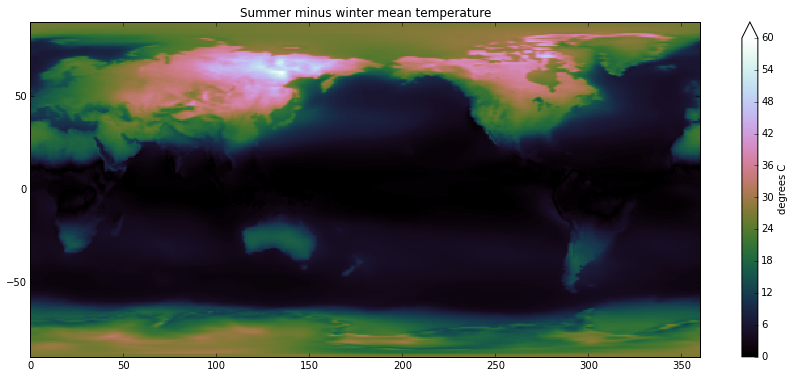

A quick aside on climate science: we see that Eastern Siberia has the world’s largest seasonal temperature swings. It is far from equator, which means that the amount of sunlight varies dramatically between winter and summer. But just as importantly, the climate is highly continental: northeast Asia is about as far away from the moderating effects of the oceans as is possible, because prevailing winds in the middle latitudes blow West to East.

The beauty of the dask.array design is that adding these operations to xray was almost no trouble at all: all we had to do is call functions like da.mean and da.concatenate instead of the numpy functions with the same names.

Computation graphs

Under the hood, dask represents deferred computations as graphs. We can look at these graphs directly to better understand and visualize our computations. Looking at these graphs also helps illustrate how dask itself works.

Here’s the graph corresponding to the above computation (limited to only two years of data). It shows how data flows as chunks through a series of functions that manipulate and combine the data, starting from files storing one month of data each:

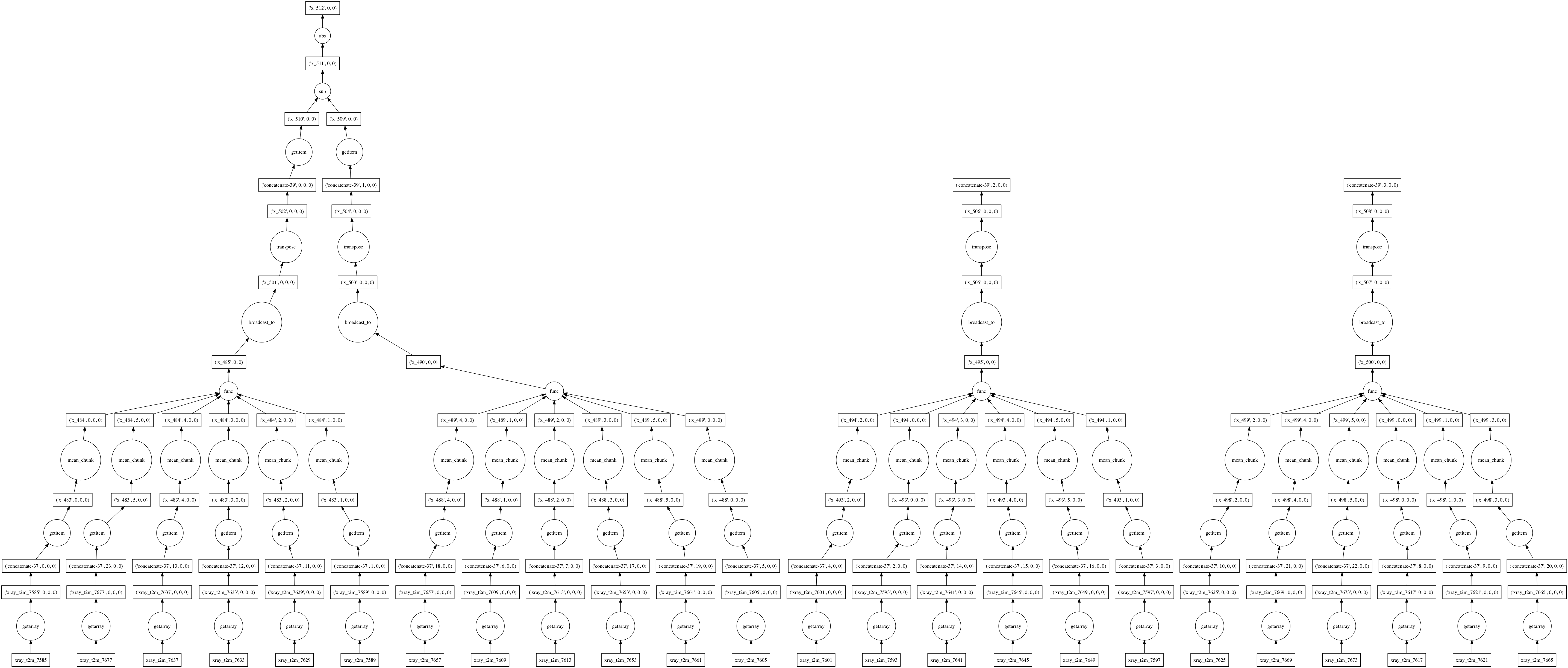
When asked for a computation result, Dask approaches graphs like this holistically. We never end up computing either of the right two branches in the above figure, corresponding to spring and fall data, because we never use them. After an optimization pass, the graph is consolidated into a much smaller set of tasks:

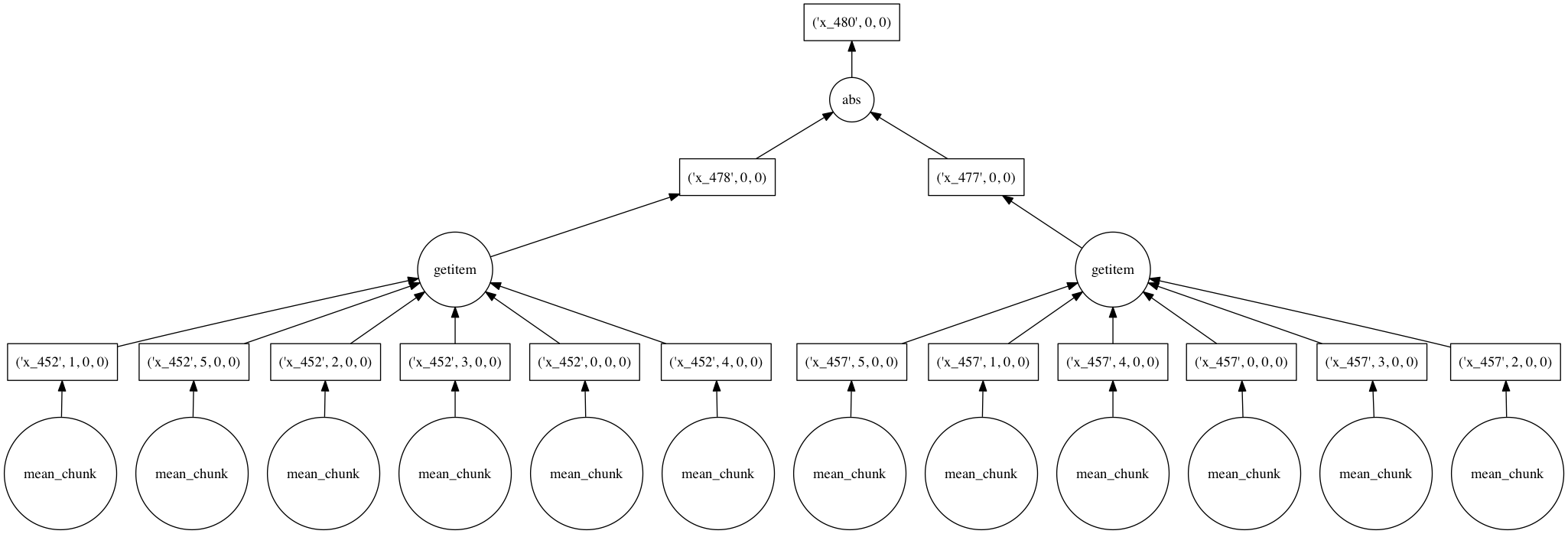
Each circle corresponds to a function evaluation on a chunk of an array handled by dask’s multi-threaded executor.

What’s next?

Last week, we released version 0.5 of xray with this experimental dask integration, giving you the features we just demonstrated. You can install it with conda:

$ conda install xray dask netcdf4

Dask will also allow us to write powerful new features for xray. For example, we can use dask as a backend for distributed computation that lets us automatically parallelize grouped operations written like ds.groupby('some variable').apply(f), even if f is a function that only knows how to act on NumPy arrays.

You can read more about what we’ve done so far in the documentation for dask.array and xray. Matthew Rocklin has recently written about the State of Dask on his blog.

If you try xray and/or dask for your own problems, we’d love to hear how it goes, either in the comments on this post or in our issue tracker.

Thanks to Matthew Rocklin, Leon Barrett, and Todd Small for their feedback on drafts of this article. It is cross posted on the Climate Engineering and Continuum blogs.